Rosenbrock函數(shù)的定義如下：

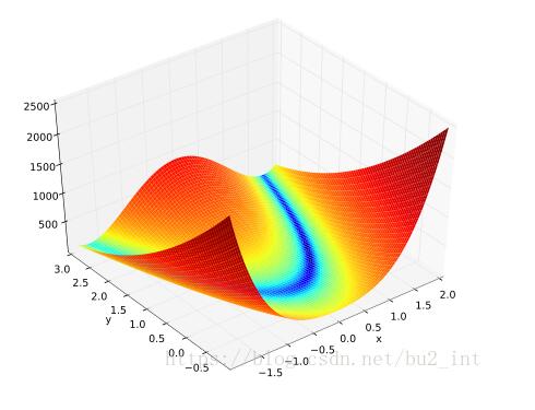
其函數(shù)圖像如下：

我分別使用梯度下降法和牛頓法做了尋找Rosenbrock函數(shù)的實(shí)驗(yàn)。

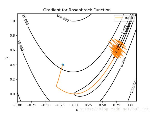
梯度下降

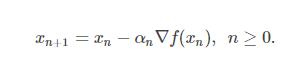
梯度下降的更新公式：

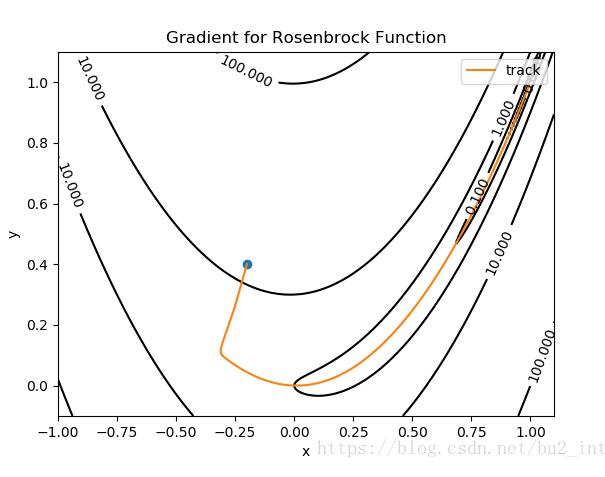
圖中藍(lán)色的點(diǎn)為起點(diǎn)，橙色的曲線（實(shí)際上是折線）是尋找最小值點(diǎn)的軌跡，終點(diǎn)（最小值點(diǎn)）為 (1,1)(1,1)。

梯度下降用了約5000次才找到最小值點(diǎn)。

我選擇的迭代步長(zhǎng) α=0.002α=0.002，αα 沒(méi)有辦法取的太大，當(dāng)為0.003時(shí)就會(huì)發(fā)生振蕩：

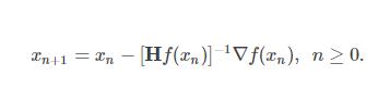
牛頓法

牛頓法的更新公式：

Hessian矩陣中的每一個(gè)二階偏導(dǎo)我是用手算算出來(lái)的。

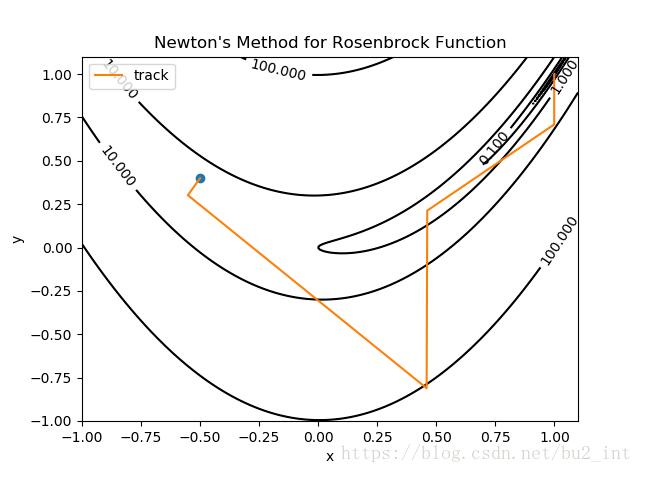
牛頓法只迭代了約5次就找到了函數(shù)的最小值點(diǎn)。

下面貼出兩個(gè)實(shí)驗(yàn)的代碼。

梯度下降：

import numpy as npimport matplotlib.pyplot as pltfrom matplotlib import tickerdef f(x, y): return (1 - x) ** 2 + 100 * (y - x * x) ** 2def H(x, y): return np.matrix([[1200 * x * x - 400 * y + 2, -400 * x], [-400 * x, 200]])def grad(x, y): return np.matrix([[2 * x - 2 + 400 * x * (x * x - y)], [200 * (y - x * x)]])def delta_grad(x, y): g = grad(x, y) alpha = 0.002 delta = alpha * g return delta# ----- 繪制等高線 -----# 數(shù)據(jù)數(shù)目n = 256# 定義x, yx = np.linspace(-1, 1.1, n)y = np.linspace(-0.1, 1.1, n)# 生成網(wǎng)格數(shù)據(jù)X, Y = np.meshgrid(x, y)plt.figure()# 填充等高線的顏色, 8是等高線分為幾部分plt.contourf(X, Y, f(X, Y), 5, alpha=0, cmap=plt.cm.hot)# 繪制等高線C = plt.contour(X, Y, f(X, Y), 8, locator=ticker.LogLocator(), colors=’black’, linewidth=0.01)# 繪制等高線數(shù)據(jù)plt.clabel(C, inline=True, fontsize=10)# ---------------------x = np.matrix([[-0.2], [0.4]])tol = 0.00001xv = [x[0, 0]]yv = [x[1, 0]]plt.plot(x[0, 0], x[1, 0], marker=’o’)for t in range(6000): delta = delta_grad(x[0, 0], x[1, 0]) if abs(delta[0, 0]) < tol and abs(delta[1, 0]) < tol: break x = x - delta xv.append(x[0, 0]) yv.append(x[1, 0])plt.plot(xv, yv, label=’track’)# plt.plot(xv, yv, label=’track’, marker=’o’)plt.xlabel(’x’)plt.ylabel(’y’)plt.title(’Gradient for Rosenbrock Function’)plt.legend()plt.show()

牛頓法：

import numpy as npimport matplotlib.pyplot as pltfrom matplotlib import tickerdef f(x, y): return (1 - x) ** 2 + 100 * (y - x * x) ** 2def H(x, y): return np.matrix([[1200 * x * x - 400 * y + 2, -400 * x], [-400 * x, 200]])def grad(x, y): return np.matrix([[2 * x - 2 + 400 * x * (x * x - y)], [200 * (y - x * x)]])def delta_newton(x, y): alpha = 1.0 delta = alpha * H(x, y).I * grad(x, y) return delta# ----- 繪制等高線 -----# 數(shù)據(jù)數(shù)目n = 256# 定義x, yx = np.linspace(-1, 1.1, n)y = np.linspace(-1, 1.1, n)# 生成網(wǎng)格數(shù)據(jù)X, Y = np.meshgrid(x, y)plt.figure()# 填充等高線的顏色, 8是等高線分為幾部分plt.contourf(X, Y, f(X, Y), 5, alpha=0, cmap=plt.cm.hot)# 繪制等高線C = plt.contour(X, Y, f(X, Y), 8, locator=ticker.LogLocator(), colors=’black’, linewidth=0.01)# 繪制等高線數(shù)據(jù)plt.clabel(C, inline=True, fontsize=10)# ---------------------x = np.matrix([[-0.3], [0.4]])tol = 0.00001xv = [x[0, 0]]yv = [x[1, 0]]plt.plot(x[0, 0], x[1, 0], marker=’o’)for t in range(100): delta = delta_newton(x[0, 0], x[1, 0]) if abs(delta[0, 0]) < tol and abs(delta[1, 0]) < tol: break x = x - delta xv.append(x[0, 0]) yv.append(x[1, 0])plt.plot(xv, yv, label=’track’)# plt.plot(xv, yv, label=’track’, marker=’o’)plt.xlabel(’x’)plt.ylabel(’y’)plt.title(’Newton’s Method for Rosenbrock Function’)plt.legend()plt.show()

以上這篇python使用梯度下降和牛頓法尋找Rosenbrock函數(shù)最小值實(shí)例就是小編分享給大家的全部?jī)?nèi)容了，希望能給大家一個(gè)參考，也希望大家多多支持好吧啦網(wǎng)。